Black Swan Farming using Cost of Delay

By Joshua J. Arnold (Black Swan Farming) and Özlem Yüce (Agile At Heart). Written in 2013 as an IEEE-format paper. This is the full paper, reformatted for the web. Original can be found and referenced here.

Abstract

Improving prioritization has become a tired concept in most IT departments, and yet it has the potential to change the conversation from one of cutting cost, to delivering valuable solutions as quickly as the business needs it. This paper examines how Maersk Line applied an economic framework across a $100 million portfolio to quickly discover, nurture and speed up the delivery of value.

Keywords: Fuzzy Front-End, Cost of Delay, Prioritisation, Value, Economics, CD3, Lean, Agile, Transformation

Contents

1. Context
2. Understanding the challenge
3. Value, flow, quality for Maersk Line
4. The case for Cost of Delay
5. Speeding up prioritisation
6. Getting to dollar benefits
7. Driving to Cost of Delay
8. Improving scheduling decisions using Cost of Delay Divided by Duration (CD3)
9. More value, faster flow, better quality
10. Finding the Black Swan
11. Conclusion
12. References
13. Notes

Context

Company

Maersk Line is the world’s largest shipping company, with 325 offices in 125 countries around the world. They have over 2.2 million containers in circulation and operate over 550 vessels [1], one of which arrives at a port on average every 15 minutes. With 18% market share and a turnover of $27 billion [2] per year, Maersk Line are the industry leader.

Culture

Using both aptitude and psychometric testing, Maersk Line hires smart people who also tend to have a high sense of urgency. They are typically process-oriented and data-driven, and they respond positively to persuasive arguments based on logic. The organization is willing to try new ways of doing things, with little resistance to change.

The organization has strong hierarchical drivers in some respects. For instance, top-down KPIs are reflected in personal objectives and performance ratings. In some aspects though, Maersk Line is a reflection of Danish culture, which is relatively open and honest. Employees are free to challenge management, exhibiting a low Power-Distance Index [3] culture. Gaining approval to change things in Maersk Line is not only a case of convincing the management layer — everyone needs to be convinced.

There is also frequent use of one of the company values: to be “upright”. This is typically interpreted as a personal responsibility to speak up if you feel others are not behaving in a way that is right for Maersk Line.

Technology

Maersk Line spends over $150m per annum on developing I.T. solutions, with over 20 development teams spread around the world. These teams are managed via a thin-outsourcing model, using the larger, more mature outsourcing vendors like IBM and TCS.

The outsourcing model means that Maersk Line expect to be able to staff their I.T. department with generalists rather than specialists. For example, it is not uncommon to make a career move from Sales to I.T.

Teams and individuals are widely distributed geographically. Colocation is not a possibility for most systems. For instance, the team for one system is spread over five locations: analysts are in Copenhagen, subject-matter-experts in Pune and a development team spread across three different time zones in the US. Average team size varies, depending on the technology, but for some systems it runs into the hundreds.

Maersk Line operates in a fairly complicated regulatory environment, intertwined with international norms and legal structures relating to who owns the contents of each container. There is a need to interface with diverse customs requirements relating to import and export regulations for each country that Maersk Line operates in. This requires local customizations and compliance to special rules about acceptable cargo types, routes, etc.

Lastly, the nature of the relationship between I.T. and the rest of the organization was highly contractual. I.T. was mostly treated as an order-taker, with relatively low trust in many areas. This made business partners somewhat suspicious of improvement ideas coming from I.T. itself. It also meant that the patience for experimenting with improvement was limited.

Understanding the challenge

We started, in October 2010, with a four-week study of the end-to-end innovation system in operation at Maersk Line. To understand how Maersk Line I.T. worked, we interviewed key stakeholders as well as people working in the teams. The study also collated and analyzed data about the value being delivered, the flow of work, and the feedback loops that drive quality.

Increasing Demand for IT

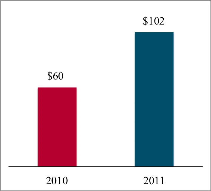
Like many organisations, Maersk Line is highly dependent on I.T. for strategic change – whether this involves making changes to existing systems or building new I.T. solutions. As a consequence, the demand for I.T. solutions had been increasing over time. This trend was reflected in the forecasted 2011 budget for software development, as shown in Figure 1. This was only an indication though – the actual demand for I.T. solutions was well in excess of this – this simply reflects what was budgeted for.

Slow delivery

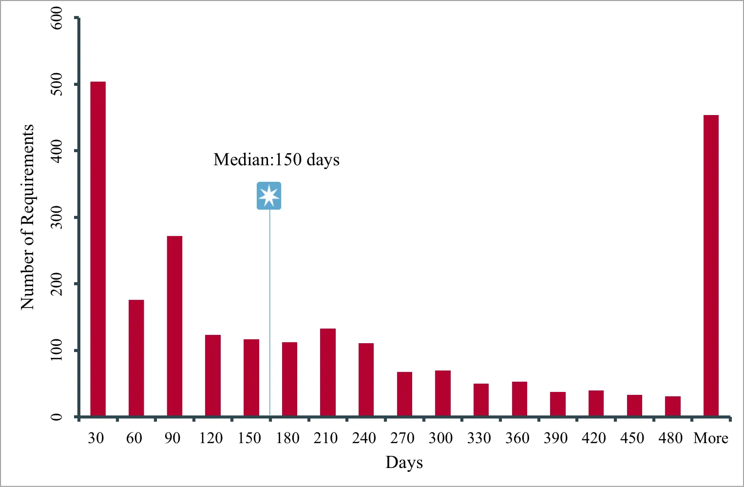
The analysis revealed that one of the most burning issues was very long end-to-end lead-time¹. In the two years prior to October 2010, it took on average 150 days to get value out of Maersk Line’s development pipeline. 24% of requirements took over a year to deliver, as shown in Figure 2.

The median lead-time was a poor reflection of the perceived speed however, with enhancements or new features² skewed to the right-hand side – where over 450 requirements took longer than 510 calendar days to deliver.

Unconstrained Work-in-Progress

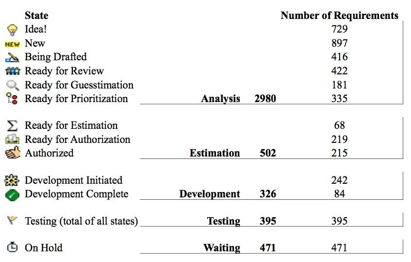
When we collected and analyzed data about work-in-progress, we could see that there was a lot of analysis and waiting time before prioritization. In particular, there were 1,856 requirements being processed between the stages of “being drafted” and “development initiated”, as shown in Figure 3. More than two-thirds of requirements were in the “fuzzy front-end”, where product development experts Preston Smith & Donald Reinertsen estimate that as much as 50% of total development time is spent [4]. An example of the fuzzy front-end at Maersk Line is shown in Figure 4.

The fuzzy front-end at Maersk Line was slow and clogged with excessive work-in-progress predominantly as a result of the funding and approval system. In order to get approval and justify funding, teams were spending time analyzing the requirements in detail up-front. In many cases, by the time the requirement was eventually authorized the analysis was obsolete due to either changes in what the customer need was, or a shift in technology. This resulted in rework, echoing W. Edwards Deming’s observation [5] about American manufacturing in his time: “Let’s make toast the American way: I’ll burn, you scrape.”

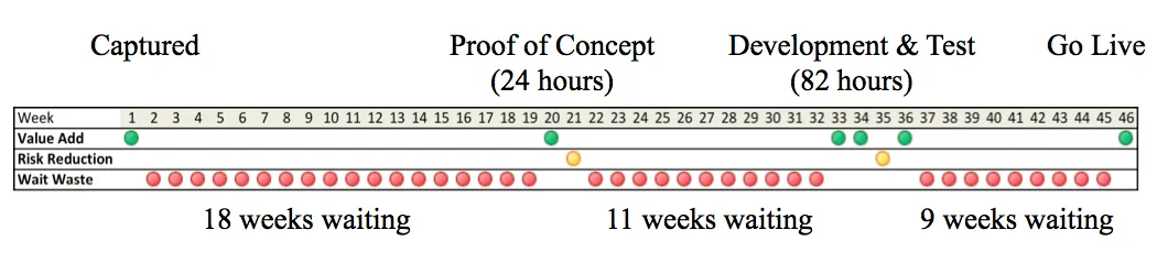
One typical example of the slow flow of work from end-to-end is illustrated in Figure 4. In this case, a feature that took only 82 hours to develop and test took a total of 46 weeks to deliver end-to-end. Waiting time ate up over 38 weeks of this. Most of this waiting time (29 weeks) was in the fuzzy front-end – where the feature was waiting in a queue to be prioritized, and then waiting again for the development work to be authorized.

Like most organisations that are blind to queues, Maersk Line were mostly focused on the efficiency of the parts of the process. The key problem here is that the efficiency of the approval process was optimized at the expense of the efficiency and speed of the end-to-end delivery of value.

Sub-Optimal Trade-offs

Maersk Line saw waste from a cost-centric view – rather than a more holistic approach that takes into account value and urgency. A strong focus on reducing development cost had resulted in sub-optimal trade-offs in decision-making. When we interviewed business stakeholders, they expressed frustration with the focus on cost reduction and the subsequent delay in deliveries.

These were some of the things we heard from business stakeholders:

“…we often save a dime to later spend a dollar”

“…a $2,000 change which took 6 weeks…”

“Saving costs is good but delivering results is better”

Value, flow, quality for Maersk Line

Alongside the interviews and analysis of data to understand the problem, we began to consider which Lean-Agile practices might help solve the problems we had seen. We narrowed down to 16 Lean-Agile practices that would fit with Maersk Line’s current reality. These were practices that could scale up to enterprise level and across the whole portfolio. They also aligned with Maersk Line’s outsourced delivery model and complex system landscape.

To get the “buy-in” to make changes, we ran a one-day workshop with the CIO and Senior Leadership Team. One of the activities involved prioritising the 16 Lean-Agile practices using the “Prune the Tree” [6] innovation game. Each practice was represented as an “apple” and the group were asked to reposition to indicate priority, with the highest priority being placed toward the root of the tree [7]. This activity increased the buy-in to each of the practices, and also helped us to build a roadmap for the change.

At the end of October, we presented the case for transformation to the two C-level executives we wanted to sponsor the initiative. We presented our findings and proposed a new approach to innovation based on Lean Product Development principles. We were given approval to go ahead and improve the end-to-end innovation system. The business case was built on three desired outcomes: more value, faster flow and better quality.

To get started with the transformation we narrowed down to 8 practices that would work for all teams. These practices were selected as those that would make meaningful impact in a relatively short time. As shown in Figure 5, we called this the “Starter Pack”. When applied together, these practices were designed to impact the whole innovation system: from the idea or “lightbulb moment” to the point when a working solution went “live”. By implementing these changes the teams would get a level of change that they could not only absorb, but also begin to see the results of working in a new way.

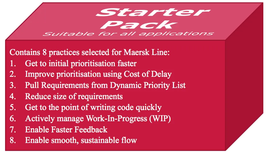
The Starter Pack was also designed to seed the transformation by demonstrating the value of a different way of working. Beyond the Starter Pack practices, the teams would embed and improve further using monthly retrospectives. To help support this we provided a simple checklist [8] of areas for teams to consider.

One of the key elements within the changes we were driving was to increase the value delivered from I.T. solutions. The aims were to improve prioritization, increase the speed of delivery and improve the visibility of trade-off decisions. Cost of Delay was at the heart of each of these.

The case for Cost of Delay

Container shipping is a highly commoditized industry that typically has excess capacity, which drives down the average price of a container [9]. In addition, demand is volatile – fluctuating based on changes in the global economy. Shipping is one of the first industries to be impacted in a downturn or recession.

To counter this, shipping companies need to move quickly. The fastest way they typically adjust is to soak up capacity by simply steaming slowly or by changing the size or number of vessels operating on a route. These tactical responses are not enough to differentiate. More strategic changes, like new routes or services can usually be copied easily by competitors. Speed to market is key to capitalizing on the few strategic opportunities that exist.

Beyond this, shipping companies look to differentiate by providing better service to their customers – and therefore increase their share of the market. Even so, improved service that is initially perceived as “delighting” quickly becomes “expected” by customers. Standing still or being slow to react is therefore a recipe for losing customers. Competing head-to-head with their competitors, with a fixed market size, is a zero-sum game³ for Maersk Line. If they are to increase the size of the market – by providing new services with new business models to new customers – they need to be able to innovate.

When it came to innovating with I.T. solutions, Maersk Line was slow. The governance process was focused on selecting the “right idea”, resulting in a very slow “front-end” process. One key reason for this was the sheer volume of ideas being analyzed in detail before the point of selection or prioritization. Moreover, we found that there was little sense of urgency to act on the ideas – even when the value was very high or when the market opportunity was time-sensitive.

This lack of urgency during the front-end of the process is related to the “Urgency Paradox” that Smith and Reinertsen discuss in their book “Developing Products in Half the Time” [10]. At Maersk Line, the urgency felt before approval was low, even when the value or market opportunity was high. Once the idea was approved and in development, the urgency felt increased (especially within I.T.). The increase in urgency happened even though the value hadn’t changed. In some cases, where the value was time-sensitive, urgency was increasing at the same time as the value was decreasing. Ignoring the impact of time on the value of ideas was costing Maersk Line.

Cost of Delay: Putting a price tag on time

In order to improve prioritization, speed up the delivery of value, and make better trade-off decisions during development, we needed a way to communicate the impact of time on value. Knowing the Cost of Delay of features helps with this.

The Cost of Delay of a feature is the value that could be generated over a given period of time, if it was available immediately. It includes the business value of the feature, the value of information that we discover as part of the development process and an assessment of how these two values decay over time.

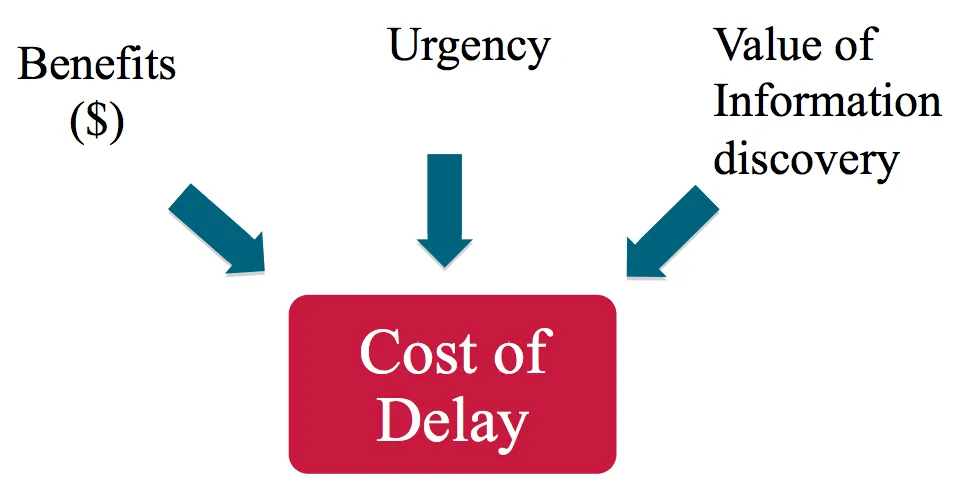
Cost of Delay is calculated by assessing the impact of not having something when you need it. As a typical example, this might be the cost incurred while waiting to deliver a solution that improves efficiency. It is the opportunity cost between having the same thing now, or getting it later.

To give a concrete example, the value-stream map shown in Figure 4 illustrates the waiting time for a real feature. In this case, the Cost of Delay for the feature was roughly $210,000 per week. This meant that the Delay Cost incurred while this feature waited in various queues for 38 weeks amounted to nearly $8 million worth of missed opportunity.

Selecting a pilot

In January 2011, we started looking at the whole system landscape in order to select a suitable candidate for piloting the “Starter Pack”. We wanted to choose somewhere that would add value, but we also wanted to learn. Despite the risks involved and the potentially long duration of implementation, we chose the Global Customer Service System (GCSS) as the first pilot. GCSS is the central booking system through which every container is booked.

GCSS is at the heart of global operation that is critical 24/7. With over 7 million lines of code, it had generated many years worth of technical debt and had almost completely manual testing. Despite the fact that it was a key dependency for almost all strategic change initiatives, making changes to this system took (on average) 373 days.

We had strong support from the Customer Service I.T. Portfolio Manager and the CTO to pilot on GCSS. One board member said to us afterwards that he “thought we were nuts” taking on GCSS. Having buy-in from I.T. wasn’t enough though; we needed to get the approval of the business. In particular, if we wanted to change the way requirements were prioritized we needed the support of the Business Process Owner (BPO) team who were responsible for feeding requirements in to I.T. This group controlled what was done and in what order. We persuaded the BPO team to give this a go: to improve prioritization using Cost of Delay.

However, we didn’t just attempt to force them to change the way they worked without offering something in return. We promised that with their help we would speed up the delivery pipeline and improve the quality – an area that they had been struggling with for many years.

By 2011, several hundred requirements had been raised for GCSS that hadn’t yet been developed (or rejected). Most of these had been briefly looked at by I.T. and given a rough sizing, or “guess-timate”, but hadn’t progressed further. The prioritization was basically binary. A requirement was either allocated to a release, and therefore “a priority” or it wasn’t. There was no “backlog” of prioritized requirements to pull from.

The initial “Dynamic Priority List”

At Maersk Line, the term “Backlog” was perceived as a negative thing. The term was associated with blocked pipes and clogged systems, causing a backlog. To avoid this, we settled on the term “Dynamic Priority List” or DPL as a replacement term for “Backlog”. This was useful in that it communicated the fact that we expected the priority list to change as new requirements were raised.

As of February 2011, there were hundreds of requirements with no estimation of value, unless they were allocated to a release. It was difficult to know where to start ordering based on value. We could have started with the oldest requirements first (First In, First Out), but this would have involved a lot of work rejecting very old or obsolete requirements. An alternative approach would have been to look at the most recent first (Last In, First Out).

Instead, the first step we took, was to prioritize the 20 requirements that had already been approved and funded for Release 23. This batch of requirements was about to enter the analysis phase, with the whole “release” batch travelling together through analysis, development, testing and deployment. These 20 requirements had already some level of analysis done in order to size them and fix the scope of the release. Before we started working with the GCSS team, they were making one release each quarter (roughly 13 weeks). The team would typically work on multiple releases at the same time, with some level of overlapping between the releases. A simplified visualization of this is shown in Figure 7.

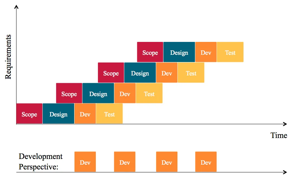
We started by randomly spreading the requirements out on a table and rearranging until they were in order of relative priority. This alone was a step toward enabling a pull system (and therefore the limiting of work-in-progress in development). Up until this time, all of the requirements that were allocated to a release were considered “priority”. In fact, when we first published an ordered list of the requirements (in order of priority) and shared this with the vendor, they didn’t understand. They thought that the whole list was “the priority” – all of them.

By the end of February, we had a new way of looking at work waiting to be done. We had managed to break the upstream batching of work⁴ and had our first of what would become many Dynamic Priority Lists.

Speeding up prioritisation

In order to attack the fuzzy front-end problem and improve the end-to-end speed, we formulated a quick triage process where teams capture ideas; evaluate cost of delay and duration. The goal was to triage all incoming requirements in less than one week. Once the requirements were triaged, they would queue in the DPL, sorted from highest priority to lowest.

The DPL needed to be a cheap place for requirements to wait until capacity became available. We didn’t want to spend a lot of time and effort getting to the DPL. To avoid analysis paralysis, the information collected during the triage process was designed to fit on one side of A5 paper. The objective was to quickly work out what the idea was roughly worth, avoiding up-front analysis.

Understanding Value

To get to the initial DPL we had already started to ask some questions about why each requirement was valuable.

To make it easier for the team to think about value, we introduced a simple framework for assessing benefits. The framework consisted of four key benefit types, or “buckets”, that a requirement might contribute to one or more of, as shown in Figure 8. The four benefit types primarily consider the likely impact on revenue and costs that a feature or project might lead to.

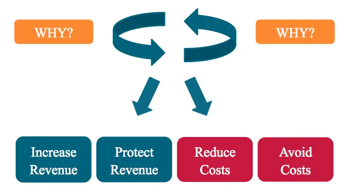
Increase Revenue

This is the revenue associated with either increasing sales to existing customers or gaining new customers. This may involve increasing share of wallet, market share or even the size of the market itself. This could be by making changes that add value to existing products or services that customers are willing to pay for, or new products or services that either existing or new customers are willing to pay for. The changes you develop here are likely to be “delighting” features for either current customers, or new ones. This is also where “disruptive innovation”⁵ occurs, enabling new business models and increasing the size of the market by serving new markets and undercutting others.

Protect Revenue

This is the revenue that is currently being received from existing customers who are paying for current products and services. Sustaining this revenue often requires ongoing improvements to at least keep up with competitors and maintain existing market share. The actions taken here are more defensive in nature, making processes faster and easier to use and removing any pain that might drive them to consider switching to a competing product or service. The changes made here are not valuable enough for existing customers to pay extra though. This is the basic maintenance of existing products and services that could be described as “sustaining innovations”⁶.

Reduce Costs

These are the ideas about how to be more efficient. The changes that contribute to this bucket will reduce the costs that we are currently incurring. Typical examples of this could be changes that speed up or automate processes, reducing the number of FTEs⁷ required. It could also result in savings in overheads, equipment or other costs.

Avoid Costs

These are costs we are not currently incurring but there is some likelihood that we will in the future, unless some action is taken. Some examples of these might be additional FTEs required to handle a new process, fines we may have to pay, or loss of reputation that impacts goodwill or brand value. This category would typically include a lot of things that many organisations might consider to be operational or strategic risks – often with an estimate of the probability of an event occurring.

Whilst we started with relative prioritization that was simply informed by thinking about the four benefit types, we wanted to go further. Our goal was more than just better prioritization for one independent pipeline. We wanted to be able to understand the impact of dependencies between pipelines. We also wanted to be able to understand which pipeline could justify increased capacity and investment to speed up end-to-end cycle time. In addition, we wanted to provide the team themselves with information about the value of the work they were doing and how that value decayed over time. They would then be in a better position to make improved trade-off decision.

To do this, we had to go beyond the simple relative prioritization. We needed to get to an estimate of the benefits expressed as a dollar value. We also needed it to be quick so that we could reduce the fuzzy front-end significantly.

Handling the HiPPO

During the initial building of the Dynamic Priority List for GCSS, we encountered the HiPPO (Highest Paid Person’s Opinion) effect. In this case the HiPPO was the most senior person in the room, with many more years of experience in the role than anyone else. The HiPPO was adamant during the initial relative prioritization that one requirement was the most valuable and urgent. With no challenge from the rest of the team it was put at the top of the DPL.

It was only when we started to go through the other 22 requirements and ask the questions we needed to get to dollar figures that we discovered that there were in fact eight other requirements that turned out to be much more valuable than the original No. 1.

This was a common story, where priorities changed as we started to uncover the real value of the features being considered – and importantly, to begin comparing them on an equal footing using the language of money. It turns out that the wisdom of a group of experts often turns out to be superior than the wisdom of one well-paid individual.

From our experience at Maersk Line, we found the HiPPO useful in the prioritization process, as it was often based on extensive knowledge of the operation and customers. In some cases though, the HiPPO completely drove the prioritization choices – with detrimental effects. The fallacy is in thinking that one person has enough knowledge of the complexity of value (or effort) involved to be able to prioritize a feature on their own. Indeed, we found it interesting how often the gut-feel and System 1⁸ thinking expressed by the HiPPO about where the value was turned out to be flawed. The HiPPO was often revealed to be mistaken by a group of experts using their combined views and had a decision framework with which to challenge the HiPPO’s priorities.

We also observed that there was a difference between what people actually knew and what they thought they knew. In his book “The Black Swan”, Nassim Nicholas Taleb calls this “epistemic arrogance” [11]. This occurs when as individuals we overestimate what we know, and underestimate uncertainty⁹.

Getting to dollar benefits

To make better prioritization decisions and make trade-offs more visible we used a simple framework and some tactics for getting to numbers that would make calculating Cost of Delay possible. Making value estimates is hard, but we believed it would be ultimately worthwhile [12]. We also felt that having a number was better than having no number at all, even if the only output was to learn more about what was valuable or not.

We were encouraged by other examples where the use of numbers was initially ignored, preferring instead to trust instinct and gut-feel. One of these was the famous story of how the Oakland Athletic baseball team completely changed the way players were picked. Rather than using the “expert” knowledge of an experienced scout (the HiPPO?), they used hard numbers about what players were observed to actually do, to select a winning team. This objective use of data, rather than subjective opinions led to the Oakland A’s going on an incredible 20-game winning streak [13]. This set a league record – despite having one of the lowest salary budgets in the baseball league. In a similar way, we wanted to question the conventional wisdom that the best way to prioritize was by deferring to a Product Owner (or HiPPO).

To get started we would evaluate each requirement against each of the four benefit types, estimating the dollar value of the benefits in each case. Assumptions were stated and made visible so that others could test the hypothesis. Using dollars had a number of advantages; the key benefit was that we were able to compare requirements immediately between business areas, across delivery streams, and the whole Maersk Line portfolio. Another driver for assigning dollar benefits to each feature was to reduce the “who shouts the loudest” that Maersk Line had suffered before. The four-bucket framework for evaluating benefits and getting to dollars also helped Business Process Owners to quickly explain why the change was important and how it would benefit the organization.

The good news is, despite our epistemic arrogance as individuals, when a group of experts collaborate they discover that they actually knew more than they thought they did. Time and time again, group after group, they went from believing that putting a dollar figure of a requirement or feature wasn’t possible – to doing it and being somewhat amazed.

Tactics for getting to numbers quickly

Getting to a dollar figure for estimated benefits can be easier than you think. Using the four benefit types triggered questions about value. When a new requirement was raised, we started by assessing the value using these four benefit types. The Lean “5-Whys” [14] technique helped us to identify the value of the requirement. We simply kept asking “why” until we were able to identify one or more of these benefit types.

We provided Business Process Owners with a couple of tactics to get to the dollar value quickly:

Estimate the beneficial effects of the change

A requirement that will generate an improvement to invoicing clarity and accuracy. If we improve invoice accuracy, customers are less likely to pay late. This would reduce the number of late payments, which would then enable us to earn interest early, hence resulting in a revenue increase.

Make the value of the requirement equal to the cost of alternatives

Let’s say we have a requirement, which will enable us to automate a process. If we automate process X, the value of the change is equal to the cost of executing process X manually.

Key questions such as “What will happen if we deliver this late?” and “What will happen if we can deliver this earlier than expected?” can drive out the answers necessary to quantify the Cost of Delay.

Making assumptions visible

Once we identified the benefit types, getting to a dollar figure typically required some assumptions about the effects of the change or the cost of alternatives. The reality of product development is that it involves many unknowns, uncertainties and probabilities. We encouraged people to make some assumptions in order to calculate the dollar benefits. This involved making educated guesses and applying probability where necessary. We explained that the goal was accuracy, not precision and that it was more important to see if we could improve knowledge and reduce our assumptions over time, based on experience. We also reiterated that the process of triaging requirements needed to be fast, less than one week.

Our rule of thumb when making assumptions was to make sure that they were made visible. This prevented blatant gaming of the benefits figures. Visibility of assumptions also allowed others to scrutinize and improve those assumptions. When we started experimenting with Cost of Delay, we arranged weekly prioritization sessions where each Business Process Owner would bring his/her requirement and the benefit case. They started reviewing the benefit cases but also the assumptions that were made when calculating the dollar benefits. They also started challenging and questioning each other about the assumptions made. Making the assumptions visible simply enabled the adjustment of the benefit calculation and the reliability of estimates improved over time, as more information was uncovered.

Another rule of thumb when making assumptions was to check whether the assumption was already used, and if it was, we made sure that we used the same numbers. We started building a repository of assumptions and key data points, which we kept sharing and building on over time.

Driving to Cost of Delay

In order to convert the benefit figures that were generated into a Cost of Delay, we needed to explain to the teams what Cost of Delay was, and why it was useful. We already had $ business value per feature. We now needed to help them understand what information discovery value meant, and how both of these decayed over time.

Information Discovery Value

Similar to many organisations, Maersk Line treated the development of solutions that didn’t work as failure – something that should be avoided – rather than recognizing the value of that information. We wanted to change this view to one that recognized that product development is a discovery process. During development we are constantly generating information about what works and what doesn’t. By putting a value on the information needed, we wanted to change the perception of value — whether the solution worked or not.

To help narrow down development options we often need to quickly test a technical or market risk. The value of doing this might be called “Information Discovery Value”. To quantify this value in a way that is comparable, we estimated the cost of both the resources and the time that we would have to otherwise spend in order to obtain the knowledge we needed.

In more simple terms, what would we be willing to pay if we could have bought the information we need? Will this architecture scale? Will this feature be used? Will this make any money for us? The answers to these questions reduce our economic risk and we should be prepared to pay something to get answers to these questions. As a result, we can at least estimate what the information is worth to us — especially to get it earlier than our competitors. Information Discovery Value is the price we would be willing to pay to discover earlier that something doesn’t work. It is the value of avoiding a long trip down the wrong path.

Urgency Profiles

In order to understand the urgency of ideas at Maersk Line, we needed to understand the life-cycle of benefits, and the effect of being late. The effect is different depending on what the benefits are, and whether it is influenced by the wider market in which Maersk Line operates.

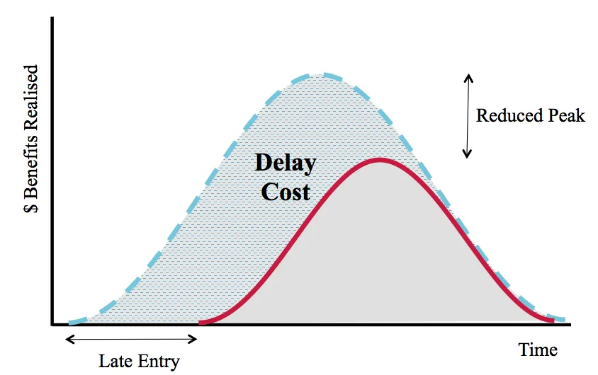
Short life-cycle; Peak affected by delay

In some cases the life-cycle of benefits is relatively short. Benefits ramp up to a peak and quickly decline again, as the value-add becomes standard for customers (rather than “delighting”) or if the market itself moves on to something different. To explain this, we gave examples of this from other industries, like fashion or other fast-moving consumer goods. With these types of benefits, if you are late, value is massively reduced, as shown in Figure 9.

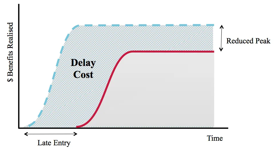
Long life-cycle; Peak affected by delay

Another urgency profile is where there is a clear first-mover advantage, making it difficult for latecomers to recover from. To illustrate, we gave examples like PC operating systems and other products or services that dominate, or where there are network effects, as shown in Figure 10. Because container shipping is mostly a commodity service, this wasn’t a common urgency profile at Maersk Line.

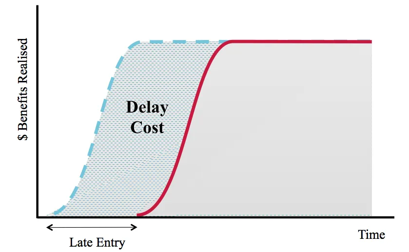
Long life-cycle, peak unaffected by delay

A third urgency profile is where the lifecycle benefits are long-lived. Benefits ramp up to a peak, and are sustained over a long period. We found this to be the most common urgency profile at Maersk Line. A typical example is where we are automating a process or improving efficiency, reducing time or cost. The ramp up and peak of benefits is effectively the same, whether the solution is late or not. This is also the easiest urgency profile for which to calculate the Cost of Delay, as it approximates nicely with a simple parallelogram as shown in Figure 11.

We used the following example to illustrate this urgency profile and how to calculate the Cost of Delay:

Requirement No: 9076

This new feature will enable automation of the invoicing process, which is expected to improve invoice accuracy. Improving invoice accuracy is expected to result in:

• Reduction in number of customers paying late, which means that the company can start earning interest. This is worth an additional $4,000,000 per annum and categorized as “Increase Revenue” benefit type.
• Reduction in number of calls currently costing 5 FTEs at $20k per FTE. This is worth $100,000 per annum and categorized as “Reduce Cost” benefit type.

Total benefit gained from this feature is equal to $4.1million per annum. Delaying this requirement by 1 week is calculated by dividing $4.1 million to 52 weeks, which is worth $78,846 per week.

If the feature were available now it would be generating $78,846 per week. If this feature was delayed by four weeks then the Delay Cost incurred is calculated as $78,846 times 4 weeks which adds up to $315,384.

Impact of External deadline

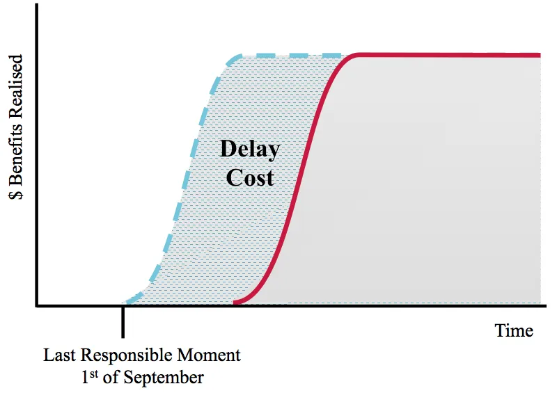
Where requirements had a specific deadline, the urgency profile and Cost of Delay was slightly more complicated. Cost of Delay only starts to ramp up as we approach the “last responsible moment”, as shown in Figure 12. To calculate the last responsible moment we need to consider the likely lead-time, ensuring that the solution is delivered just-in-time, rather than too early or too late.

Requirement No: 9077

There is a new regulation that will be effective from 1^st of December 2013. As of December, customer service will need to prepare extra documentation in order to meet this regulation. This requirement is to automate the new documentation process so that the customer service employees could produce the documentation automatically.

The requirement will avoid the additional manual processing resource, which is estimated to cost about 20 FTEs at $20k per FTE. The benefit type is categorized as “Avoid Cost”.

20FTE × $20k= $400,000 per annum

Let’s say it is 1st of June 2013 right now, which means we have got 5 months to do something about this requirement. It’s going to take about 13 weeks¹⁰ to deliver this new feature. If we start developing the solution now it will be delivered in September but we don’t need it until later.

We deal with this by calculating the last responsible moment of when we need to start developing the solution. The last responsible moment is calculated by subtracting the duration from the external deadline. In this case the last responsible moment for starting development is 1^st of September (calculated by subtracting 13 weeks from the external deadline of 1st of December). Until the last responsible moment of 1st of September, the Cost of Delay for this requirement is zero, which then rises beyond the last responsible moment.

Beyond the last responsible moment of 1^st of September 2013, Cost of Delay is equal to;

$0.4m/52 weeks = $7,692 per week

These examples were effective in demonstrating how Cost of Delay could be calculated within the context of the shipping industry. They helped Business Process Owners to start calculating the Cost of Delay for the requirements they were raising.

Improving scheduling decisions using Cost of Delay Divided by Duration (CD3)

On its own, having a better understanding of Cost of Delay improved the visibility of value and urgency. One of the key benefits though is when we used Cost of Delay to improve prioritization. With increasing demand for I.T. solutions and limited ability to increase capacity, the senior leadership team were very interested in learning how to leverage Cost of Delay to control demand better and deliver more value.

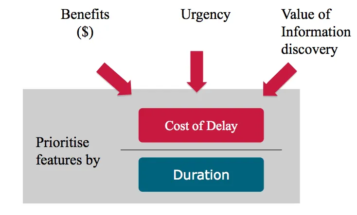
We started using CD3 – Cost of Delay Divided by Duration¹¹ – to schedule work. The priority order of features or projects was determined by dividing the estimated Cost of Delay by the estimated duration, as shown in Figure 13: the higher the resulting score, the higher the priority. To explain how this approach increased the value delivered, we compared it with alternative scheduling methods.

Comparing CD3 with FIFO

In order to demonstrate how CD3 improves prioritization we compared CD3 to the different scheduling methods using simple scenarios.

Feature	Cost of Delay	Duration (weeks)	CD3
A	$1/week	5	0.2
B	$4/week	1	4
C	$5/week	2	2.5

Let’s assume we have 3 features in our DPL: Feature A, B and C. Cost of Delay for A is $1/week, Cost of Delay for B is $4/week and the Cost of Delay for C is $5/week. Duration of A, B and C are respectively 5 weeks, 1 weeks and 2 weeks.

Using these three features let’s have a look into the impact of two alternative scheduling methods.

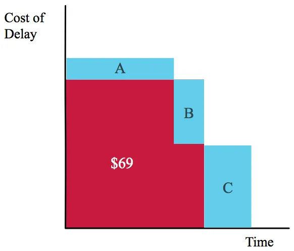
One option is to use the “First In First Out” (FIFO) method to schedule work. This is a method that is widely used in manufacturing and the purpose is to serve the customers in the order that they arrive. If we apply the FIFO method to schedule above features, we would work on these three features one at a time in the order they arrived. The person asking for Feature A will have been waiting for the longest time so FIFO scheduling method suggests that we deliver Feature A first, then Feature B, and finally Feature C.

Feature A will take 5 weeks to deliver. When the team is working on Feature A, Delay Cost incurred is equal to the sum of Cost of Delay of all three features times by duration of A.

Delay Cost incurred when delivering Feature A
= (CoD_A + CoD_B + CoD_C) × Duration_A
= ($1/week + $4/week + $5/week) × 5
= $50

Delay Cost incurred is $50 during the time it takes to develop Feature A.

Once the team delivers Feature A, they then move on to developing Feature B. When Feature B is being delivered, Delay Cost incurred is equal to the sum of the Cost of Delay of Feature B and Feature C times duration of Feature B.

Delay Cost incurred when delivering Feature B
= (CoD_B + CoD_C) × Duration_B
= ($4/week + $5/week) × 1
= $9

During the time it takes the team to deliver Feature B, the Delay Cost is an additional $9.

Lastly, once Feature B is delivered, team starts working on Feature C. While the team is working on Feature C, the Delay Cost incurred is equal to the Cost of Delay of Feature C times duration of Feature C.

Delay Cost incurred when delivering Feature C
= CoD_C × Duration_C
= $5/week × 2
= $10

During the time it takes the team to deliver Feature C, the Delay Cost is an additional $10.

When we sum the Delay Cost incurred during development of each feature, total Delay Cost adds up to $69 as shown in Figure 15.

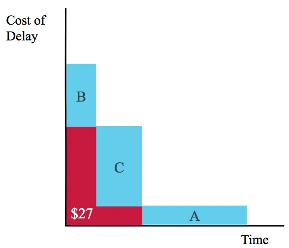
If we sequence the delivery based on whichever has the highest CD3 score the team would develop Feature B first, followed by Feature C, and finally Feature A.

When the team is working on Feature B, Delay Cost incurred is equal to $10.

Delay Cost incurred when delivering Feature B
= (CoD_B + CoD_C + CoD_A) × Duration_B
= ($4/week + $5/week + $1/week) × 1
= $10

When the team is working on Feature C, Delay Cost incurred is equal to $12.

Delay Cost incurred when delivering Feature C
= (CoD_C + CoD_A) × Duration_C
= ($5/week + $1/week) × 2
= $12

Lastly, when the team is working on Feature A, Delay Cost incurred is equal to $5.

Delay Cost incurred when delivering Feature A
= CoD_A × Duration_A
= $1/week × 5
= $5

Delay Cost over 8 weeks when using CD3 scheduling method adds up to $27, as shown in Figure 16 – resulting in a 60% reduction in the total Delay Cost compared to FIFO method.

Making Adjustments to CD3

We realized that prioritization would not always be made purely based on numbers. We used additional levers such as Business and I.T Strategy when necessary. To handle this we used a “raw” CD3 score as an initial means of triage and allowed the teams to adjust the score (up or down) by making a plus or minus adjustment of the Cost of Delay (not the CD3 score directly). The amount of adjustment and the reason for adjustment were then made visible to everyone. We also encouraged teams to make a short note, so that others would understand why the adjustment had been made.

Decisions were still made by people but using CD3 lead to improved prioritization and helped teams make the right decisions with the right information.

More value, faster flow, better quality

By July 2011, we were starting to see measurable improvements in a number of areas. This was not solely down to the implementation of Cost of Delay and CD3, but from all of the Starter Pack practices. By the time we started to see results, we had already been rolling out changes to the rest of the portfolio and two core systems, GCSS and FACT/SAP had the following results.

Faster Flow: Improvement in Speed of Delivery

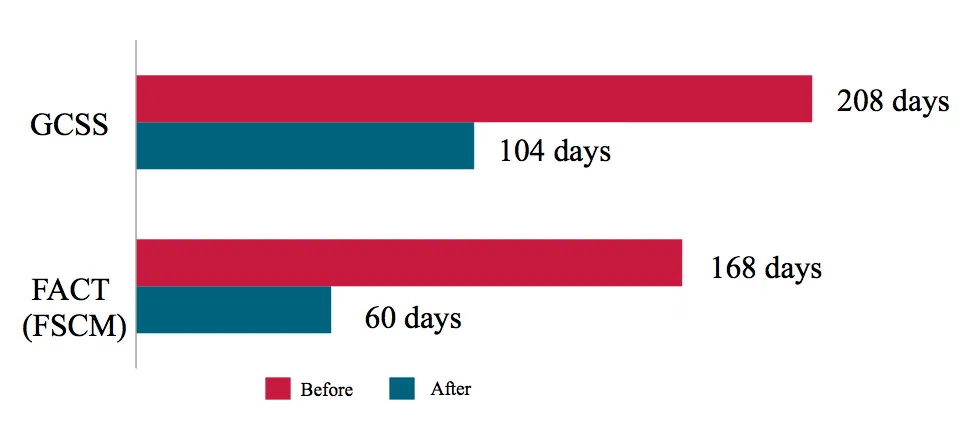
The cycle time from DPL to production for GCSS reduced from an average of 208 days, down to an average of 108 days. For the centralized SAP finance and accounting system “FACT” the full end-to-end lead time reduced from 168 days down to 60 days on average. The halving of the cycle time can be seen in Figure 17.

Improving prioritization using Cost of Delay and CD3 played a key role in improving the speed of delivery mainly due to two reasons:

• Cost of Delay creates urgency and this sense of urgency encourages actions, which are focused on reducing time-to-market of I.T. solutions.
• As CD3 uses “duration” on the denominator, it encourages the breakdown of work into smaller batches. Increasing the batch size leads to a penalty in terms of priority, so it drives the right behavior – to break the work down. For example, if you can identify the 20% of effort that will deliver 80% of the value then the priority increases by a factor of four. Breaking work down into smaller batches is one of the easiest and most powerful improvements that can be made in order to speed up delivery of value and improving end-to-end flow of requirements.

Better Quality: Customer Satisfaction

Another area where we saw improvements was in the internal “Voice of the customer” survey, which was measured every two months. In particular, GCSS team saw a significant improvement, going from one of the worst results across Maersk Line – both below average and below target – to above average and above target, as shown in Figure 18.

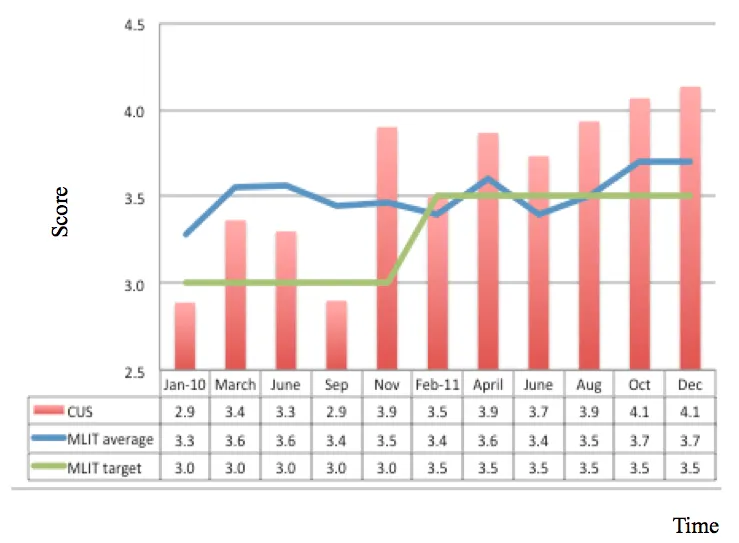
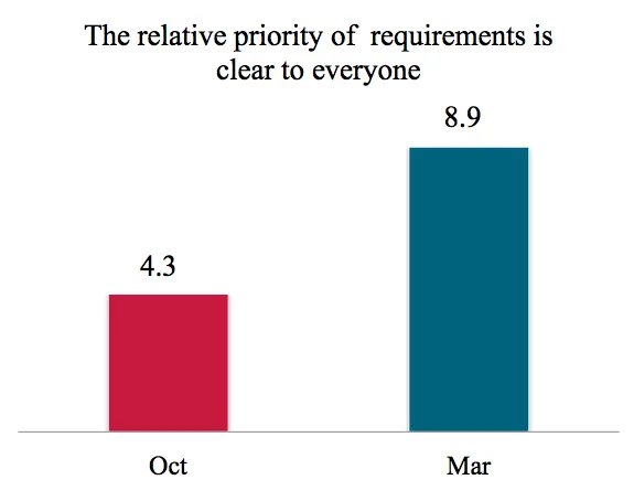
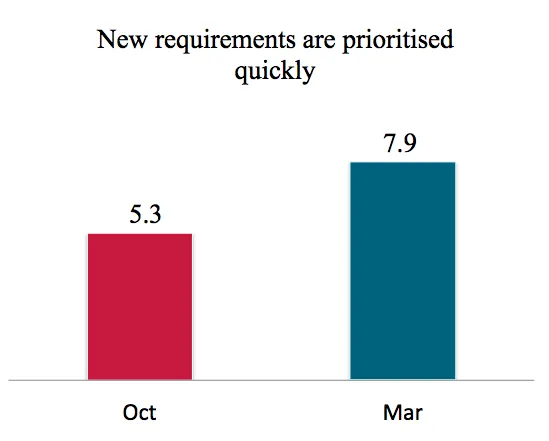
The same effect was seen for the FACT delivery team. In particular, there were four questions that we were interested in, as shown in Figure 19 and Figure 20. Two questions were in particular related to Cost of Delay and CD3. As you can see that the average response to the statement “The relative priority of requirement is clear to everyone” improved from 4.3 to 8.9 and the average response to the statement “New requirements are prioritized quickly” improved from 5.3 to 7.9.

Peter Hartz, one of the Business Process Owners shared his view about the improvements made.

“The main difference we have seen in the BPO department since we started using Cost of Delay is that we have a better framework for prioritising requirements. We started talking about the most valuable and urgent changes for the company, instead of ‘my changes’. The framework helps us to challenge requirements that come in regardless of which party submits the requirement. It puts us, the BPO team, in a better position to challenge each other and gives us better visibility of the priorities. Lastly, and most important of all, it reduced the lead time of the prioritized requirements tremendously, helping us to react faster to the market and customer demands.”

Peter Hartz, Business Process Owner, Maersk Line

More Value: Increase in the visibility of benefits

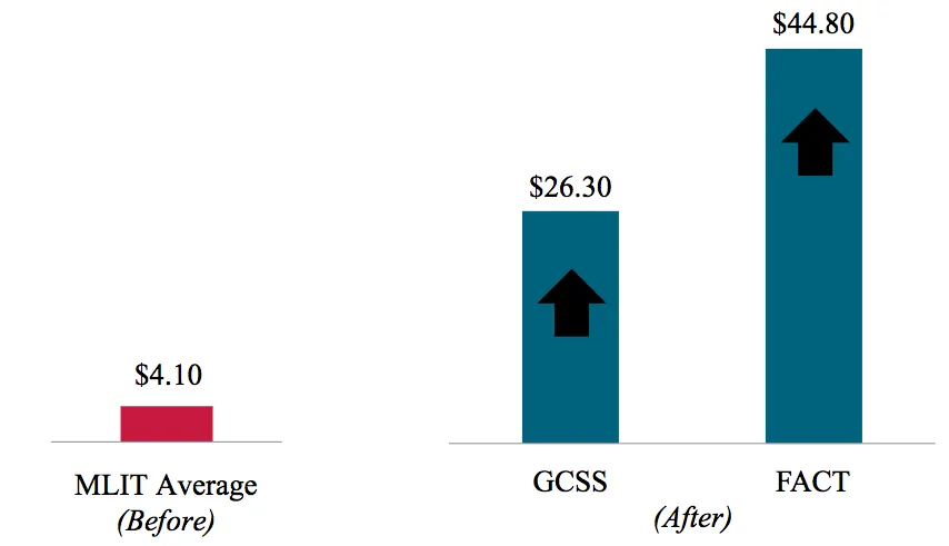
Prior to implementation of Cost of Delay and CD3, there was no tracking of Return on Investment (ROI) per system or per feature. The average Return on Investment from I.T. solutions across Maersk Line was $4.1¹², which can be seen in Figure 21. When we compare the average ROI from GCSS and FACT features delivered to the ROI of Maersk Line, it was a massive improvement. Average ROI of GCSS features were 6 times higher compared to Maersk Line average and 11 times higher for FACT features that were delivered.

More Value: Clear prioritisation across the portfolio

We were able to use Cost of Delay and CD3 effectively within a single project or I.T. system but the benefits of use across projects and programs were more effective. When applied across the whole portfolio, Cost of Delay and CD3 created a clear focus on priorities across the whole business. This simplified decisions about what was most valuable for the organization by increasing the visibility of the cost of work and the benefits of that work.

This is what the Head of the Business Process Owner team said about improving prioritization using Cost of Delay and CD3:

“… less yelling and screaming, data-driven, more visible”

Head of the Business Process Owner team, Maersk Line

Another benefit of using Cost of Delay and CD3 is that it provided clarity on urgency between different pieces of work and helped handle dependencies across different teams.

More Value: Enabling better Trade off decisions

Making Cost of Delay visible enabled the conversation to change from delivering on time, or cutting costs, to delivering value quickly. Cost of Delay provided a guide to the urgency of the requirement; it challenged those involved to think in terms other than minimizing cost, forcing them to question how to maximize value and finally assisted in decisions in terms of how the solution to the requirement is delivered.

Better Quality: Speeding up feedback

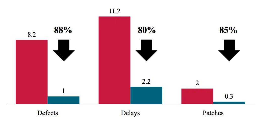
By speeding up existing feedback loops, introducing new feedback loops where they were missing, and bringing some of them forward in the process we saw a dramatic 88% reduction in the number of defects. The delays experienced with previous GCSS releases were typically related to quality issues – so seeing this reduce by 80% was another indicator of the improvement in quality. Lastly, when major problems were discovered between releases, this would usually require patching. We saw the number of patches required reduce by 85%, a huge improvement, not to mention the cost and risks involved in doing this. These quality improvements are shown in Figure 22.

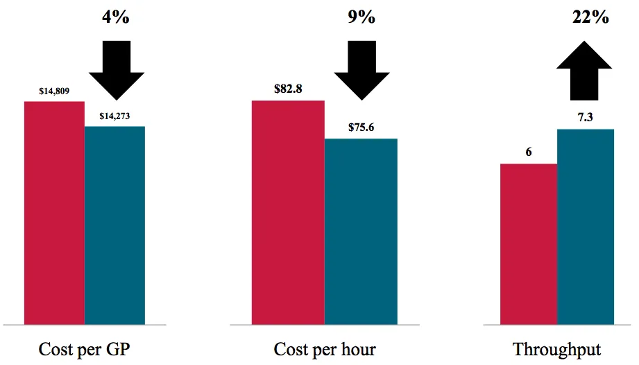
(While we were not at all focused on reducing costs or increasing throughput, one interesting result we saw was the increase in throughput by 22% and a small reduction in cost. This is shown in Figure 23).

Finding the Black Swan

As we expected, the Cost of Delay of requirements at Maersk line was far from being equal, or evenly distributed. What we really weren’t expecting to discover was just how rare the most valuable requirements were. Finding the value in Maersk Line’s Dynamic Priority Lists was like hunting for Black Swans¹³.

The distribution of Value

For instance, when we looked at the Cost of Delay for the most valuable and urgent 25% of requirements in the DPL for GCSS, they were worth three orders of magnitude more than the bottom 25%, as shown in Figure 24. Not ten times, or one hundred times, but a thousand times more valuable.

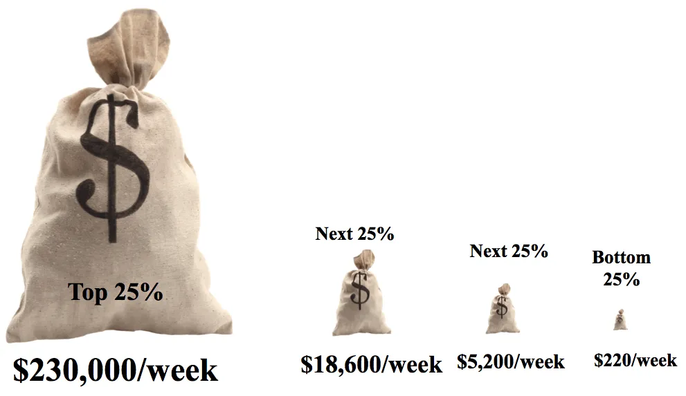
This suggests that if Maersk Line were to use a four-category prioritization system for GCSS, like MoSCoW¹⁴, that the top “must-have” category would be worth ten times more than the “could-have” category, and one thousand times more than the lowest category.

When we plotted a distribution of the Cost of Delay of the GCSS requirements we saw that the distribution fit a typical “Pareto distribution” power-law curve, as shown in Figure 25.

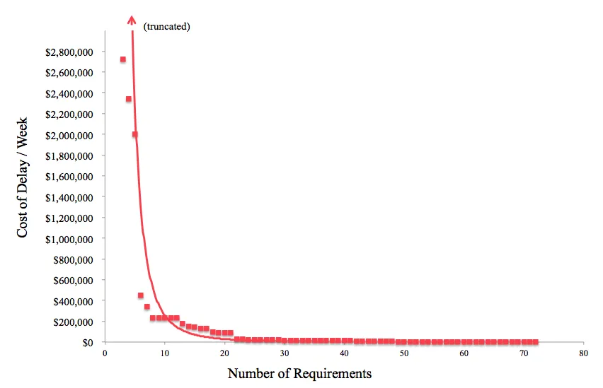
We saw the same distribution of Cost of Delay when we looked at the requirements for the SAP Finance system. This is shown in Figure 26.

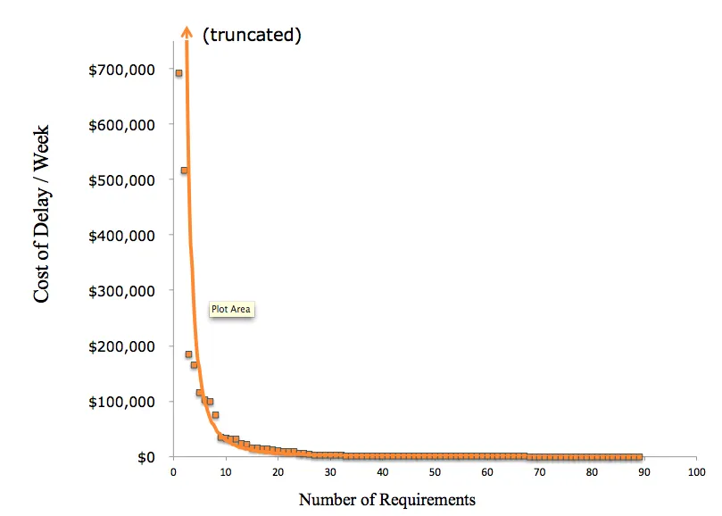
Within the FACT requirements, even when we considered the subset of the requirements raised by Damco¹⁵ – who had to pay for each of their requirements – the distribution of Cost of Delay again fitted the now familiar Pareto power-law curve. The distribution of value for Maersk Line is shown as the orange curve in Figure 27. Damco is the red curve.

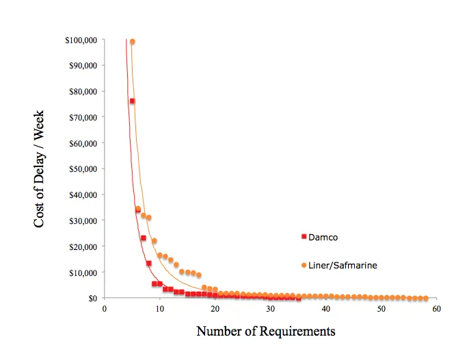
Just like Vilfredo Pareto¹⁶, who observed that 20% of the pea pods in his garden contained 80% of the peas, we observed a similar distribution of the Cost of Delay in the Dynamic Priority Lists of a global shipping giant. This result held true even for relatively small sets of requirements, showing that the power-law relationship was scale-invariant.

The problem with “Projects”

Seeing the evidence of this suggested that it really was worth the effort to break work down and consider value at the feature level. What this also suggests is that projects are a poor vehicle for delivering valuable software. By attributing value to the whole project, rather than individual features, this effectively waters down the benefit cost ratio of the most valuable features. It becomes easier to batch up and hide a bunch of low-value features inside the project alongside the “vital few” that are truly valuable, forcing them to carry the others. This is a classic batch size problem.

Using projects at Maersk Line had other effects though. By fixing the duration of projects, the organization missed the high Cost of Delay ideas that arrived after the pre-defined window of opportunity had closed. Even worse, was when they not only fixed the duration of the project but also attempted to fix the scope prior to approval. This had the effect of reducing even further the window of opportunity. The incentive for the business was to try and work out up-front what the whole solution “needed” to be. Unfortunately, most of what gets included at this point has a low Cost of Delay – a truly sub-optimal approach. In effect, projects at Maersk Line were a tail-dropping FIFO queuing system – one that tended to ignore late arriving, but high Cost of Delay ideas. Our conclusion is that projects are a poor vehicle for improving how the organization works as well as the products and services they provide.

Value is rare, extreme and obvious in retrospect

Nassim Nicholas Taleb describes “Black Swans” as rare events; that have an extreme impact; and that appear obvious only in retrospect. When viewed through the lens of value and urgency, there were a very small number of ideas for which the impact on the organization was extreme. Yet this was not obvious until the economic value and urgency was considered. We found that within the pool of ideas generated at Maersk Line there were what we would characterize as Black Swans.

The point about being “obvious only in retrospect” is an important one when it came to the Cost of Delay calculations themselves – but perhaps more importantly, management’s view of the numbers produced. The typical response, which we heard more than once at Maersk Line, was the desire to “hold people to account” for their value estimates. In fact, we heard various ideas about how to punish or reward the individuals or groups raising ideas, depending on whether their idea turned out to be as valuable as they had predicted.

Doing this would have had a negative impact though, driving the organization back to being risk averse and slow when evaluating benefits. Business Process Owners would be incentivized to only raise ideas where they could be sure of the result, like headcount reductions or other cost saving. Focusing only on reducing cost becomes a zero-sum game. At some point, the organization needs to also focus on creating value for its customers, and in doing so increase the size of the market.

The reality is, innovation and product development are not sure things. It is more like what venture capital firms do – a series of small bets, some of which will hopefully pay for all the others. They attempt to pick winners, but they are still hostage to the market and the probability of success is low. Much the same as with the banking system, none of the bets we make should ever become “too big to fail”. Innovation requires that we test new ground and break things, discovering the best solution. Probe, sense, respond: Amplify the positive signal, dampen the negative signal. In this way, product development is not so much Black Swan hunting, but more like Black Swan farming.

Projects hide a lot of these small bets though and provide management with a false sense of control. You actually have more visibility and control when you deliver a series of small incremental and iterative steps, ordered by CD3. We were amazed by the concerns that some managers shared about this approach. They seemed to be worried that delivering features quickly would steal focus from the big, important and strategic projects. Conventional thinking suggests that the way to achieve a big vision is to set up big projects. Unfortunately, the truth is the opposite: that there has been high correlation between project size and failure [15].

Why not just build the most valuable 25%?

What would the result be if only the most valuable 25% ever got built? The problem is: 25% of what, exactly? Of the originally planned requirements? Of all the requirements ever raised? For all of the systems at Maersk Line, the number of “requirements” was growing. This is a good thing. Not all of the ideas we first have about how to improve our organization are the most valuable. Some of the ideas we are going to have in the next 12 months will have a very high Cost of Delay. One definition of a project is: “[a..] planned set of interrelated tasks to be executed over a fixed period and within certain cost and other limitations” [16]. This is why projects, by the typical definition, are a sub-optimal way of building valuable software.

Because of the non-linear distribution of value in the DPLs at Maersk Line, we suggested that they should focus on building small sustainable teams oriented around products or services. A key part of the recommendation was to keep the teams together and make sure they have everything they need in order to deliver quickly end-to-end. Maintain a focus on quickly delivering no more than 10% of the initial view of what is needed, but allow the requirements to continue flowing in – and then apply Cost of Delay and CD3 to find the “Black Swan” features that were really valuable and urgent.

If the list of requirements, and the priority of them does not change over time, then teams would be highly likely to end up building features for which the expected economic value was low.

Should we focus on discarding 80% of requirements?

At Maersk Line, there was a lot of focus and effort put into saying “no”. The problem with this was that this ends up being more like a high-jump than a binary yes/no. The result being that even more time and effort was put into analyzing the requirements and building a business case (or a political case) for doing the work.

We have seen that saying “no” is hard. Better to just avoid the need to say “no” and focus more on saying “yes” quickly to the really valuable ideas that are revealed during triage. Storing the low-value ideas is cheap. Better to divert the resource that is typically incentivized to keep pushing the same idea. Instead, ask them to focus on breaking down and providing feedback on the ideas you want to quickly explore and build. In our experience, it’s just not worth the effort of trying to say “no”.

Conclusion

In 2010, Maersk Line set out to fundamentally change the way it innovated. By implementing 8 selected Lean-Agile practices across their portfolio, they delivered more value, faster flow, and better quality I.T. solutions.

With more focus on value, Business Process Owners used a simple framework to quickly evaluate ideas. This faster triage process reduced the work-in-progress and significantly sped up the fuzzy front-end.

By expressing benefits in dollars Maersk Line was better able to compare the value of ideas coming from different parts of the organization, as well as handle dependencies between different teams more easily. Taking into account how that value decayed over time for each idea facilitated better understanding of the Cost of Delay.

As Don Reinertsen says: “If you only measure one thing, measure the Cost of Delay” [17]. The plethora of trade-off decisions could now be informed by an understanding of value and how sensitive to time that value was.

Cost of Delay also created a sense of urgency about the ideas being developed and made the case for optimizing the end-to-end flow of work, (rather than optimizing parts of the flow).

Using Cost of Delay and CD3 to prioritize and schedule the development of ideas increased the visibility and granularity of value for the organization. Return on Investment increased to $26 per dollar invested for the centralized global booking engine and $44 per dollar invested for the centralized finance and accounting system. Since CD3 divides by duration, it also incentivized the breaking down of work, a key driver of value, flow and quality. The improvements meant that Maersk Line were more focused on the most value-adding work, with CD3 providing a clear way of handling the ever increasing demand that I.T. departments so often struggle with.

The results were surprising, especially given the change was mostly in how they worked rather than in the engineering. The end-to-end cycle time for delivering features was reduced by 50% for the centralized global booking engine, from 208 days down to 104 on average. For the centralized SAP finance and accounting system the improvements in flow were even more stark, going from 168 days down to 60 days on average.

On the quality side, by introducing new feedback loops and speeding up others, the number of defects, delays and patches fell dramatically for the centralized booking engine.

Most organisations intuitively believe that expressing benefits at feature level is too difficult or time consuming. It turns out that this isn’t as hard as you think, and can be done quickly — far quicker than the usual fuzzy front-end for projects. And it is really worthwhile making the effort for a number of reasons. Our experience challenges the accepted norm of defaulting to a single Product Owner (or the Highest Paid Person’s Opinion) when it comes to estimating value and choosing priority order. Our experience leads us to believe that projects are a poor vehicle for delivering valuable software. Part of the reason for this is the clear evidence that the distribution of value in our backlogs is far from linear. The most valuable 25% can be worth over a thousand times more than the least valuable 25% with the distribution of value following a Pareto power-law curve. We need to be looking for and discovering the rare, extreme value features, for which the value will seem obvious only after the fact: Black Swans.

Acknowledgements

We would like to thank everyone at Maersk Line and Emergn involved in the initiative. In particular, the Lean Product Development team without whom we wouldn’t have a story worth telling: Chris Berridge, Fredrik Hagstroem, Jorge Migueis, Matt Steen, Lisa Doa, Steve Eadie, Tom Sedge.

References

[1] Online at http://www.maerskline.com/link/?page=brochure&path=/about_us

[2] Henrik Brunniche Lund, Stephanie Fell, “A.P. Moller- Maersk A/S Group, Annual Report 2012”, Online at http://files.shareholder.com/downloads/ABEA-3GG91Y/2534603720x0x637633/183d2a61-4bed-4afd-a142-d723121da6f8/Presentation_Annual_Report_2012.pdf, 2013

[3] “Power Distance Index”, Online at http://www.clearlycultural.com/geert-hofstede-cultural-dimensions/power-distance-index/

[4] Preston G. Smith, Donald G.Reinertsen, “Developing Products in Half the Time”, John Wiley and Sons, New York, 1998, pp. 50-51

[5] David S. Greisler, “William Edwards Deming: The Man”, Journal of Management History, Vol. 5, No. 8, 1999, pp. 434-453

[6] Innovation games, “Prune the Product Tree”, Online at http://innovationgames.com/prune-the-product-tree/

[7] Joshua J. Arnold, “A History of Value, Flow and Quality”, Online at http://costofdelay.com/a-history-of-value-flow-and-quality/, 2013

[8] Chris Berridge, Joshua J. Arnold, “Lean Product Development Checklist”, Online at http://costofdelay.com/lean-product-development-checklist/, 2013

[9] Jens Søndergaard, Lars R. Eismark, Jan Bovermann, “Balancing the Imbalances in Container Shipping”, Online at http://www.atkearney.com/paper/-/asset_publisher/dVxv4Hz2h8bS/content/balancing-the-imbalances-in-container-shipping/10192, 2012

[10] Preston G. Smith, Donald G.Reinertsen, “Developing Products in Half the Time”, John Wiley and Sons, New York, 1998, pp.53-54

[11] Nassim Nicholas Taleb, “The Black Swan”, Penguin Books, 2011, pp. 138-141

[12] Joshua J. Arnold, “Why making value estimates is hard but worthwhile”, Online at http://costofdelay.com/why-making-value-estimates-is-hard-but-worthwhile/, 2013

[13] “Oakland Athletics Seasons”, Online at https://en.wikipedia.org/wiki/2002_Oakland_Athletics_season

[14] “5Whys technique”, Online at https://en.wikipedia.org/wiki/5_Whys

[15] C. Verhoef, “Quantitative IT portfolio management”, Online at http://www.cs.vu.nl/~x/ipm/ipm.pdf, Elsevier Science B.V., 2002, pp. 45

[16] Online at http://www.businessdictionary.com/definition/project

[17] Donald G. Reinertsen, “The Principles of Product Development Flow: Second Generation Lean Product Development”, Celeritas Publishing, 2009, pp.31

Notes

¹ We have defined lead-time as the elapsed time from “lightbulb” to “live”. We measured this from the time an idea was captured to the time when it was deployed and working in production. ↩

² We defined a “feature” as the smallest unit of independently deliverable business value. Delivering a part of a feature does not deliver any business value. As a general rule, we found that features could be smaller than what people generally think. ↩

³ A “zero-sum game” is a situation where the sum of the gains and losses of all the participants will be equal to zero. Someone has to lose for someone to win. ↩

⁴ We also needed to change the funding and approval process to fit with a pull system – as discussed briefly here: http://costofdelay.com/systems-thinking-and-i-t/ ↩

⁵ Disruptive innovation aims to create a new market and value network, but over time disrupts an existing market and value network. ↩

⁶ Sustaining innovation aims to make existing market or value networks better to sustain improvements. It is not about creating new markets or value networks. ↩

⁷ Full-Time Equivalent, which means one employee working full-time. ↩

⁸ The theory that Daniel Kahneman won a Nobel Prize for is based on the contrast between two fundamentally different ways of thinking: System 1 is fast, based on instinct and what we feel; System 2 is slower, more considered, analytical and informed by logic. ↩

⁹ We do this by reducing the number of possible uncertain states that we consider. We limit our thinking to primarily what we know, and in the process leave ourselves exposed to known unknowns and unknown unknowns. ↩

¹⁰ 13 weeks is calculated based on the worst-case lead-time for developing and deploying the solution. Then we considered the frequency of the releases to have an estimation of the duration. ↩

¹¹ CD3 is a specific form of the “Weighted Shortest Job First” scheduling method. We renamed it to CD3 to put more emphasis on Cost of Delay (the value part) – instead of how long or short the job was ↩

¹² Source: Belinda Qvist, Maersk Line Strategic Projects. This was the benefit cost ratio for all of the releases tracked by Maersk Line Strategic Projects in 2009. ↩

¹³ According to the Black Swan theory, black swans are rare and improbable events that are outliers beyond the realm of expectations. ↩

¹⁴ Prioritisation method based on categorizing requirements as “must-have”, “should-have”, “could-have”, and “would-have”. Indicating that “must have” requirements are top priority. ↩

¹⁵ Damco is supply chain management and logistics company, which is owned by A.P. Moller-Maersk Group. ↩

¹⁶ Vilfredo Pareto was an Italian economist, after whom the Pareto Principle is named. ↩